One of the most popular trends today is to be “data-driven”. But what does that mean? It means that you make your strategic business decisions using the data you collect, or pay for. However, data in its raw form is rarely useful. To make sense of it, you need data analysts who can draw insights from the collected data. Well, before analysts can do their job, you need to store that data somewhere, and preferably in a way that will make the analyst’s job easier. 

At our company, we use mostly Celery and Airflow for building data pipelines and we store (ingest) the data into Big Query tables. Airflow is a work orchestration tool whose pipelines are called DAGs (Directed Acyclic Graphs). Each DAG consists of a number of operators (also called tasks). So, basically, a data pipeline consists of a series of tasks that read, transform and store data. 

One of our DAGs has worked fairly well for the last 10 months. It ran every morning. Occasionally, the pipeline (DAG) would fail. It wasn’t a notable issue – we would just clear the DAG run and the pipeline would restart. However, recently the issue started occurring more frequently and it was time to address it. 

The operator that would fail in the DAG is responsible for copying the data from a Postgres table into Big Query. What the operator internally does, it dumps the data from the production database into a csv file and uploads it to Big Query. However, the operator started to fail more frequently with a timeout exception. 

When a query times out, and it isn’t your database, there are basically two things that you can try:

Simplify/optimise the query

Split the data into batches and handle each batch separately. 

Optimising the Query

The query we used was fairly simple:

Now, the important thing to mention here is that columns 1 and 2 contain JSON data. I came upon a blog post or stackexchange/stackoverflow question which mentioned that we could get better performance in Postgres if we query only the field that we need. 

So, let’s take a look at the data in our columns:

Column1 – json has 5 fields, 2 of which interest us;

Column2 – json has around 25 fields, 3 of which interest us.

That seems like a large discrepancy. Now, I didn’t take the average size of each json field in the table rows. This would be a good approach if you need to see how much you may save on memory or storage size. In my case, I took a look at only the values in a single row, just to get the feeling about the size. Of course, looking at a single row might be misleading, and might lead you to draw the wrong conclusions if you accidentally chose an anomalous row in the table. 

But from the one example, I noticed that the 3 fields we are interested in are simple arrays that will have a limited number of values. Some other fields seem to be arrays of json values. 

So, I constructed a query that would take only the fields from the json values that we need:

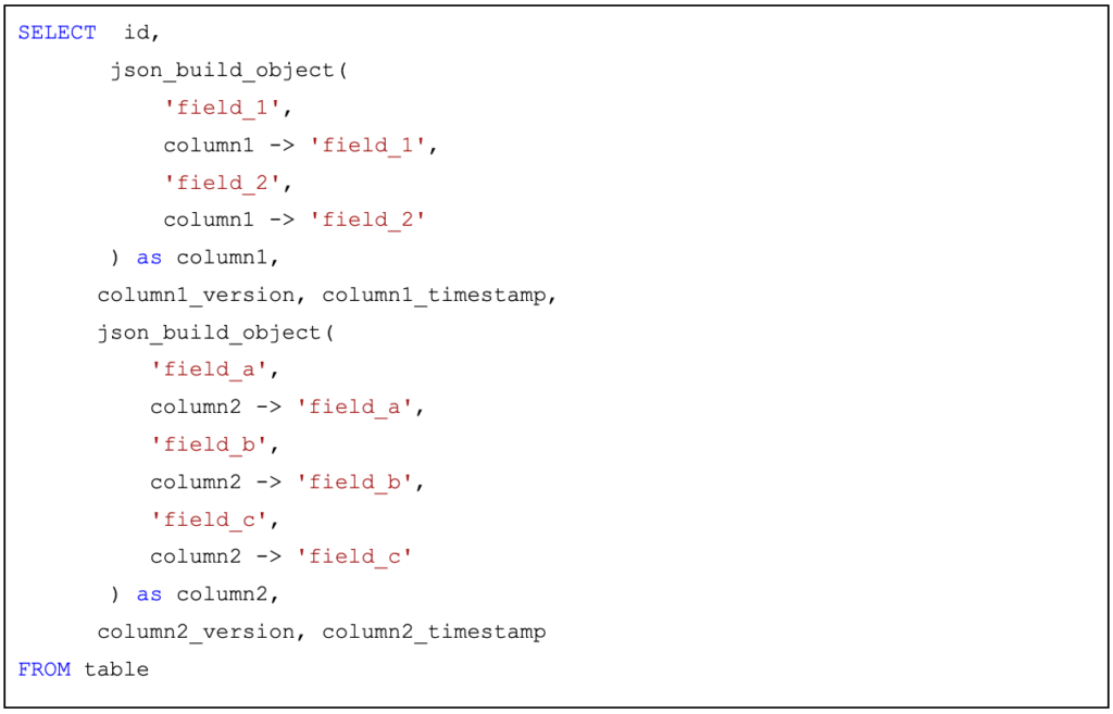
Notice the json_build_object function. I’m using this to construct a new json object with the same keys as the json in the columns to achieve backward compatibility. I’m also giving the columns the appropriate name. With these two things in place, the next operator in the DAG will receive the values in an expected schema.

The next step was to run the queries in DataGrip and see how they perform (I limited them both to 80 000 rows):

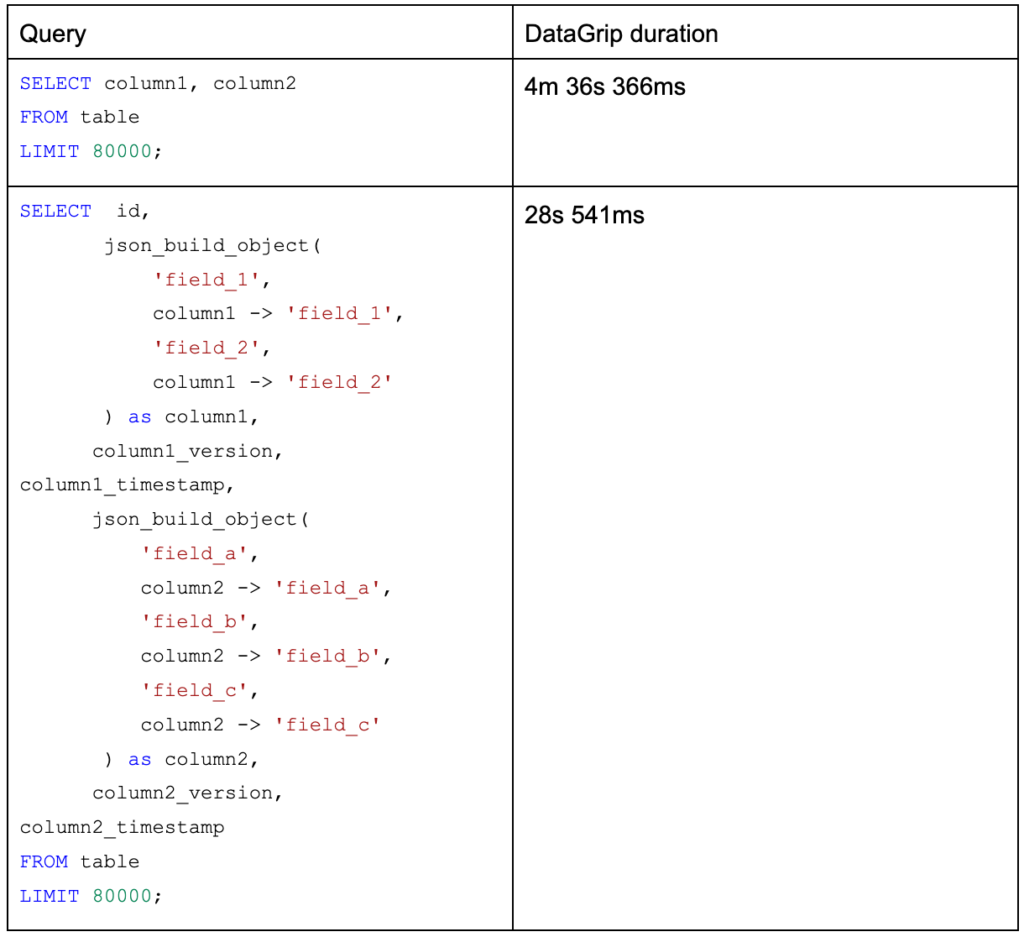
This table indicates that the second query is several times faster. Of course, a single run is not a good indicator of query performance. It could have been that there was network latency when running one of the queries, or the production database experienced greater load. 

In order to compare the speed of using these two queries in Python, I created a small script. I wanted to compare these two queries when querying the entire database 10 times for different batch sizes. 

However, it took too long. For the query in the second row (the faster one) it took around 20 minutes to query the entire table. That means that given 10 iterations, it would take about 200 minutes, or 3 and a half hours. The query in the first row (the slower one) takes even more time to get the data. I assume around 6 hours, although I didn’t test it. I concluded that carrying out this kind of investigation on a personal computer just isn’t feasible. Note: some of this latency is due to VPN – we can’t connect to the database without it. 

It occurred to me that I could bring up a local instance of the database and use that for testing. But the entire table has more than 9GBs of data. So, I didn’t like that option. 

Therefore, I decided to run each query 10 times, but query only a single batch  (80 000 rows) of data from the table, and use that to compare the speed of the queries. The table below shows the durations (in seconds) taken from the test:

The data clearly shows that the more complex query is several times faster.

Here is the code that was used:

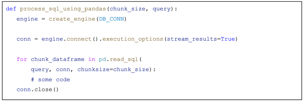
I found the example here: https://pythonspeed.com/articles/pandas-sql-chunking/

However, since this querying happens in an Airflow operator, I proposed that we try to implement the solution using airflow’s Hooks. 

Query in batches

The other thing we can do is to query only a subset of the data and do that as many times as we need (as long as the owner’s of the database don’t kill us for making too many connections). A good batch_size is something you have to determine for yourself. If you can test a number of different batch sizes over more than 10 iterations, you could get a good idea of which batch size is best suited for you. For us, a good batch size seemed to be somewhere between 50 000 and 100 000. There are almost 800 000 rows in the table we query.

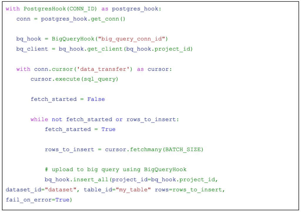
The code would look something like this:

Summary

In summary, the proposed solution consists of two steps:

Use the faster version of the query:

Drawbacks: not all of the fields will be copied and potentially may one day need to add them

Split the reading of data into fixed size batches. 

We would need a PythonOperator which would call a function that would read the data from PostgreSQL and write it to Big Query. To achieve this, you can use PostgresHook and BigQueryHook. 

Looking at the implementation of PostgresHook, it is possible to create a server-side cursor to fetch the data. Why server-side cursor? Because we do not want to load an extensive amount of data into Airflow.

A server side cursor is created when a name for the cursor is passed to the cursor factory method. 

Future work

Hopefully, one day we will upgrade to Airflow 2.4 (at least). Once that happens, we will have the ability to create dynamic tasks. That means that we will be able to have an operator that will not need to loop over all of the rows in the table. Rather, we will be able to dynamically create X task instances and have each of them collect a piece of the data.

An example:

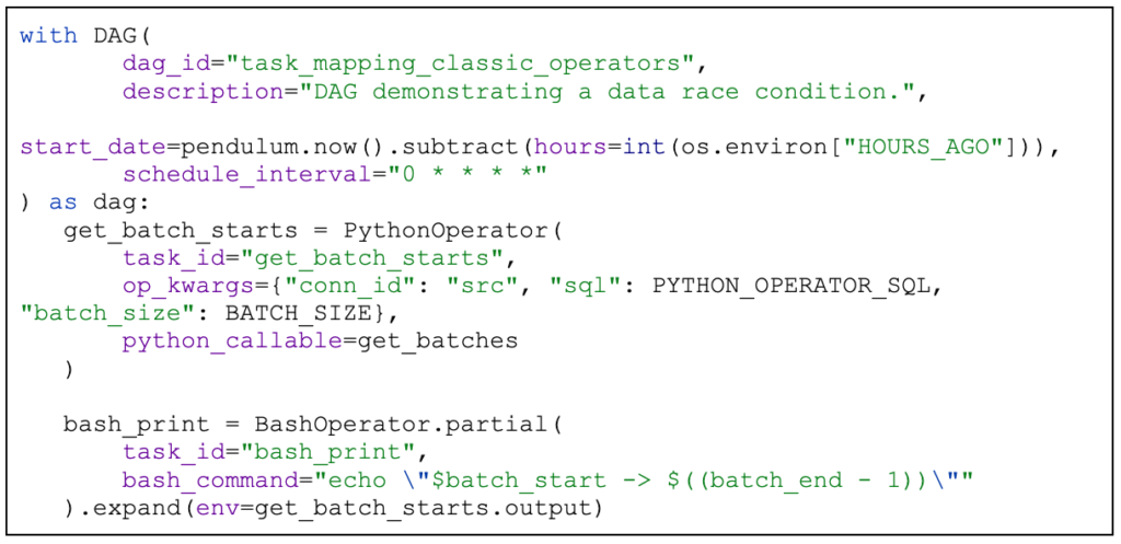
The important part here are the partial and expand functions. The partial function declares a partial operator. The expand function tells the scheduler to create a single task instance for each element of the list passed to env parameter.